Hi there!

This is a place where I store my notes.

这个地方存放了我的笔记。

Algorithms

• CodeTop Solutions
• CodeWar Selections

Useful links:

• https://en.cppreference.com/w/cpp/algorithm
• https://en.cppreference.com/w/cpp/container

CodeTop

3. 无重复字符的最长子串

class Solution {
public:
    int lengthOfLongestSubstring(string s) {
        vector<int> idx(128, -1);
        int l = 0, ans = 0;
        for (int r = 0; r < s.size(); r ++) {
            if (idx[s[r]] >= l) {
                l = idx[s[r]] + 1;
            }
            idx[s[r]] = r;
            ans = max(ans, r - l + 1);
        }
        return ans;
    }
};

146. LRU缓存机制

class Node {
public:
    int k, v;
    Node *pre, *nex;
    Node() : k(0), v(0), pre(nullptr), nex(nullptr) {}
    Node(int _k, int _v) : k(_k), v(_v), pre(nullptr), nex(nullptr) {}
};

class LRUCache {
    Node *head, *tail;
    int cap;
    unordered_map<int, Node *> store;

public:
    LRUCache(int capacity) : cap(capacity) {
        // dummy head & tail
        head = new Node();
        tail = new Node();
        head->nex = tail;
        tail->pre = head;
    }

    int get(int key) {
        if (!store.count(key)) {
            return -1;
        }
        Node *n = store[key];
        moveToHead(n);
        return n->v;
    }

    void put(int key, int value) {
        if (store.count(key)) {
            Node *n = store[key];
            n->v = value;
            moveToHead(n);
            return;
        }
        if (store.size() >= cap) {
            Node *toRemove = tail->pre;
            store.erase(toRemove->k);
            removeNode(toRemove);
        }
        Node *n = new Node(key, value);
        moveToHead(n);
        store[key] = n;
    }

    void removeNode(Node *n) {
        n->pre->nex = n->nex;
        n->nex->pre = n->pre;
    }

    void moveToHead(Node *n) {
        if ((n->pre && n->pre->nex == n) || (n->nex && n->nex->pre == n)) {
            removeNode(n);
        }
        n->pre = head;
        n->nex = head->nex;
        head->nex->pre = n;
        head->nex = n;
    }
};

206. 反转链表

/**
 * Definition for singly-linked list.
 * struct ListNode {
 *     int val;
 *     ListNode *next;
 *     ListNode() : val(0), next(nullptr) {}
 *     ListNode(int x) : val(x), next(nullptr) {}
 *     ListNode(int x, ListNode *next) : val(x), next(next) {}
 * };
 */
class Solution {
public:
    ListNode* reverseList(ListNode* head) {
        ListNode *pre = nullptr;
        ListNode *cur = head;
        while (cur) {
            ListNode *next = cur->next;
            cur->next = pre;
            pre = cur;
            cur = next;
        }
        return pre;
    }
};

215. 数组中的第K个最大元素

class Solution {
public:
    int findKthLargest(vector<int>& nums, int k) {
        int n = nums.size();
        int minVal = *min_element(nums.begin(), nums.end());
        int maxVal = *max_element(nums.begin(), nums.end());
        vector<int> bucket(maxVal - minVal + 1, 0);
        for (int i = 0; i < n; i++) {
            bucket[nums[i] - minVal]++;
        }
        // 每个桶可能不止一个
        int count = 0;
        for (int i = bucket.size() - 1; i >= 0; i--) {
            count += bucket[i];
            // 这个桶加完后超过 k 表示已经找到了
            if (count >= k) {
                return i + minVal;
            }
        }
        return -1;
    }
};

25. K 个一组翻转链表

/**
 * Definition for singly-linked list.
 * struct ListNode {
 *     int val;
 *     ListNode *next;
 *     ListNode() : val(0), next(nullptr) {}
 *     ListNode(int x) : val(x), next(nullptr) {}
 *     ListNode(int x, ListNode *next) : val(x), next(next) {}
 * };
 */
class Solution {
public:
    ListNode* reverseKGroup(ListNode* head, int k) {
        if (head == nullptr) return head;
        int i = k;
        ListNode *cur = head;
        while (cur && --i > 0) { // --i，提前一格退出，那么 cur 指向最后一个
            cur = cur->next;
        }
        // no more than k;
        if (cur == nullptr) return head;
        ListNode *nextHead = cur->next;
        ListNode *pre = nullptr;
        cur = head;
        while (cur != nextHead) {
            ListNode *tmp = cur->next;
            cur->next = pre;
            pre = cur;
            cur = tmp;
        }
        head->next = reverseKGroup(nextHead, k);
        return pre;
    }
};

15. 三数之和

class Solution {
public:
    vector<vector<int>> threeSum(vector<int>& nums) {
        sort(nums.begin(), nums.end());
        vector<vector<int>> ans;
        for (int k = 0; k < nums.size() - 2; k++) {
            if (nums[k] > 0) break;
            if (k > 0 && nums[k] == nums[k - 1]) continue;
            int l = k + 1, r = nums.size() - 1;
            while (l < r) {
                int sum = nums[l] + nums[r] + nums[k];
                if (sum == 0) {
                    ans.push_back({nums[l], nums[r], nums[k]});
                    while (l < r && nums[l] == nums[++l]); // && nums[l] == nums[++l] 先加 l + 1，然后跳过所有相等的
                    while (l < r && nums[r] == nums[--r]); // 同上
                }
                if (sum < 0) 
                    while (l < r && nums[l] == nums[++l]);
                if (sum > 0) 
                    while (l < r && nums[r] == nums[--r]);
            }
        }
        return ans;
    }
};

53. 最大子数组和

class Solution {
public:
    int maxSubArray(vector<int>& nums) {
        int dp = nums[0];
        int ans = nums[0];
        for (int i = 1; i < nums.size(); i ++) {
            dp = max(dp + nums[i], nums[i]);
            ans = max(dp, ans);
        }
        return ans;
    }
};

补充题4. 手撕快速排序

class Solution {
public:
    vector<int> sortArray(vector<int>& nums) {
        quick_sort(nums, 0, nums.size() - 1);
        return nums;
    }

    void quick_sort(vector<int>& nums, int l, int r) {
        if (l < r) {
            int pivot = partition(nums, l, r);
            quick_sort(nums, l, pivot - 1);
            quick_sort(nums, pivot + 1, r);
        }
    }

    int partition(vector<int>& nums, int l, int r) {
        int key = nums[l];
        while (l < r) {
            while (l < r && nums[r] >= key) r --;
            nums[l] = nums[r];
            while (l < r && nums[l] <= key) l ++;
            nums[r] = nums[l];
        }
        nums[l] = key;
        return l;
    }
};

21. 合并两个有序链表

/**
 * Definition for singly-linked list.
 * struct ListNode {
 *     int val;
 *     ListNode *next;
 *     ListNode() : val(0), next(nullptr) {}
 *     ListNode(int x) : val(x), next(nullptr) {}
 *     ListNode(int x, ListNode *next) : val(x), next(next) {}
 * };
 */
class Solution {
public:
    ListNode* mergeTwoLists(ListNode* list1, ListNode* list2) {
        ListNode* dummy = new ListNode();
        ListNode* cur = dummy;
        ListNode* cur1 = list1;
        ListNode* cur2 = list2;
        while (cur1 || cur2) {
            if (!cur1) {
                cur->next = cur2;
                cur = cur->next;
                cur2 = cur2->next;
                continue;
            }
            if (!cur2) {
                cur->next = cur1;
                cur = cur->next;
                cur1 = cur1->next;
                continue;
            }
            if (cur1->val < cur2->val) {
                cur->next = cur1;
                cur = cur->next;
                cur1 = cur1->next;
            } else {
                cur->next = cur2;
                cur = cur->next;
                cur2 = cur2->next;
            }
        }
        return dummy->next;
    }
};

5. 最长回文子串

class Solution {
public:
    // dp[i, j] = dp[i + 1, j - 1] && (s[i] == s[j])
    string longestPalindrome(string s) {
        bool dp[1009][1009];
        int maxAns = 0;
        int l = 0;
        // 注意递推方程的性质，i 依赖 i + 1，j 依赖 j - 1
        for (int j = 0; j < s.length(); j++) {
            for (int i = 0; i <= j; i++) {
                if (i == j) {
                    dp[i][j] = true;
                } else if (i == j - 1 && s[i] == s[j]) {
                    dp[i][j] = true;
                } else {
                    dp[i][j] = dp[i + 1][j - 1] && s[i] == s[j];
                }
                if (dp[i][j] && j - i + 1 > maxAns) {
                    maxAns = j - i + 1;
                    l = i;
                }
            }
        }
        return s.substr(l, maxAns);
    }
};

102. 二叉树的层序遍历

/**
 * Definition for a binary tree node.
 * struct TreeNode {
 *     int val;
 *     TreeNode *left;
 *     TreeNode *right;
 *     TreeNode() : val(0), left(nullptr), right(nullptr) {}
 *     TreeNode(int x) : val(x), left(nullptr), right(nullptr) {}
 *     TreeNode(int x, TreeNode *left, TreeNode *right) : val(x), left(left), right(right) {}
 * };
 */
class Solution {
public:
    vector<vector<int>> levelOrder(TreeNode* root) {
        vector<vector<int>> ret;
        if (!root) {
            return ret;
        }
        queue<TreeNode *> q;
        q.push(root);
        while (!q.empty()) {
            int currentLevelSize = q.size(); // 这里得保存，不然在 for 循环中 q 会持续变大
            ret.push_back(vector<int>());
            for (int i = 1; i <= currentLevelSize; ++i) {
                auto node = q.front();
                q.pop();
                ret.back().push_back(node->val);
                if (node->left) q.push(node->left);
                if (node->right) q.push(node->right);
            }
        }
        return ret;
    }
};

1. 两数之和

class Solution {
public:
    vector<int> twoSum(vector<int>& nums, int target) {
        unordered_map<int, int> numMap;
        int n = nums.size();
        for (int i = 0; i < n; i++) {
            int complement = target - nums[i];
            if (numMap.count(complement)) {
                return {numMap[complement], i};
            }
            numMap[nums[i]] = i;
        }
        return {};
    }
};

33. 搜索旋转排序数组

class Solution {
public:
    int search(vector<int>& nums, int target) {
        int n = nums.size();
        int l = 0, r = n - 1;
        while (l <= r) {
            int mid = (l + r) / 2;
            if (nums[mid] == target) return mid;
            // 检查 mid 在哪个有序区间内
            if (nums[0] <= nums[mid]) {
                // 第一个有序区间内，检查是否可以缩减到 0 ~ mid 范围内
                if (nums[0] <= target && target < nums[mid]) {
                    r = mid - 1;
                } else {
                    l = mid + 1;
                }
            } else {
                // 第二个有序区间内，检查是否可以缩减到 mid + 1 ~ n - 1 范围内
                if (nums[mid] < target && target <= nums[n - 1]) {
                    l = mid + 1;
                } else {
                    r = mid - 1;
                }
            }
        }
        return -1;
    }
};

200. 岛屿数量

class Solution {
int direction[4][2] = {{0, 1}, {1, 0}, {-1, 0}, {0, -1}};
public:
    // 常规写法
    int numIslands(vector<vector<char>>& grid) {
        int ans = 0;
        bool mark[300][300];
        memset(mark, 0, sizeof(mark));
        for (int i = 0; i < grid.size(); i++) {
            for (int j = 0; j < grid[i].size(); j++) {
                if (grid[i][j] == '0' || mark[i][j]) {
                    continue;
                }
                dfs(mark, grid, i, j);
                ans++;
            }
        }
        return ans;
    }

    void dfs(bool mark[300][300], vector<vector<char>>& grid, int i, int j) {
        if (i < 0 || j < 0 || i >= grid.size() || j >= grid[i].size() ||
            grid[i][j] == '0') {
            return;
        }
        if (mark[i][j]) {
            return;
        }
        mark[i][j] = true;
        for (auto& d : direction) {
            int di = d[0];
            int dj = d[1];
            dfs(mark, grid, i + di, j + dj);
        }
    }
};

46. 全排列

class Solution {
public:
    vector<int> vis;
    vector<int> path;

    void dfs(vector<vector<int>>& ans, vector<int>& nums, int x) {
        if (x >= nums.size()) {
            ans.push_back(path);
            return;
        }
        for (int i = 0; i < nums.size(); i++) {
            if (vis[i]) continue;
            vis[i] = 1;
            path.push_back(nums[i]);
            dfs(ans, nums, x + 1);
            vis[i] = 0;
            path.pop_back();
        }
    }

    // 回溯板子题，来自题解 dfs 暴搜，排列组合
    vector<vector<int>> permute(vector<int>& nums) {
        vector<vector<int>> ans;
        vis.resize(nums.size(), 0);
        dfs(ans, nums, 0);
        return ans;
    }
};

20. 有效的括号

class Solution {
public:
    bool isValid(string s) {
        stack<char> t;
        for (char c : s) {
            if (c == '(' || c == '{' || c == '[') {
                t.push(c);
                continue;
            }
            if (t.empty()) {
                return false;
            }
            char l = t.top();
            t.pop();
            if (c == ')' && l != '(') return false;
            if (c == ']' && l != '[') return false;
            if (c == '}' && l != '{') return false;
        }
        return t.empty();  // 最后的栈一定是空的
    }
};

121. 买卖股票的最佳时机

class Solution {
public:
    // O(N)
    // 先有股票最低点，然后才有可能有比之前还多的利润
    int maxProfit(vector<int>& prices) {
        int buy = 0, profit = 0;
        for (int i = 0; i < prices.size(); ++i) {
            if (prices[i] < prices[buy]) {
                buy = i;
            }
            int gain = prices[i] - prices[buy];
            if (gain > profit) {
                profit = gain;
            }
        }
        return profit;
    }
};

88. 合并两个有序数组

class Solution {
public:
    // 常规写法
    void merge(vector<int>& nums1, int m, vector<int>& nums2, int n) {
        vector<int> ans;
        int i = 0, j = 0;
        while (i < m || j < n) {
            if (j >= n) {
                ans.push_back(nums1[i]);
                i++;
                continue;
            }
            if (i >= m) {
                ans.push_back(nums2[j]);
                j++;
                continue;
            }
            if (nums1[i] <= nums2[j]) {
                ans.push_back(nums1[i]);
                i++;
            } else {
                ans.push_back(nums2[j]);
                j++;
            }
        }
        copy(ans.begin(), ans.end(), nums1.begin());
    }
};

103. 二叉树的锯齿形层序遍历

/**
 * Definition for a binary tree node.
 * struct TreeNode {
 *     int val;
 *     TreeNode *left;
 *     TreeNode *right;
 *     TreeNode() : val(0), left(nullptr), right(nullptr) {}
 *     TreeNode(int x) : val(x), left(nullptr), right(nullptr) {}
 *     TreeNode(int x, TreeNode *left, TreeNode *right) : val(x), left(left), right(right) {}
 * };
 */
class Solution {
public:
    vector<vector<int>> zigzagLevelOrder(TreeNode *root) {
        vector<vector<int>> ans;
        if (!root) {
            return ans;
        }
        queue<TreeNode *> q;
        q.push(root);
        bool flag = false;
        while (!q.empty()) {
            vector<int> l;
            int lsize = q.size();
            for (int i = 0; i < lsize; i++) {
                TreeNode *f = q.front();
                q.pop();
                l.push_back(f->val);
                if (f->left) q.push(f->left);
                if (f->right) q.push(f->right);
            }
            if (flag) {
                reverse(l.begin(), l.end()); // 反转
                flag = false;
            } else {
                flag = true;
            }
            ans.push_back(l);
        }
        return ans;
    }
};

141. 环形链表

/**
 * Definition for singly-linked list.
 * struct ListNode {
 *     int val;
 *     ListNode *next;
 *     ListNode(int x) : val(x), next(NULL) {}
 * };
 */
class Solution {
public:
    bool hasCycle(ListNode *head) {
        unordered_set<ListNode *> s;
        while (head) {
            if (s.count(head)) {
                return true;
            }
            s.insert(head);
            head = head->next;
        }
        return false;
    }
};

// TODO: 快慢指针

236. 二叉树的最近公共祖先

/**
 * Definition for a binary tree node.
 * struct TreeNode {
 *     int val;
 *     TreeNode *left;
 *     TreeNode *right;
 *     TreeNode(int x) : val(x), left(NULL), right(NULL) {}
 * };
 */
class Solution {
public:
    TreeNode* lowestCommonAncestor(TreeNode* root, TreeNode* p, TreeNode* q) {
        if (root == q || root == p || !root) return root;
        TreeNode* left = lowestCommonAncestor(root->left, p, q);
        TreeNode* right = lowestCommonAncestor(root->right, p, q);
        if (left && right) return root;
        if (!left) return right;
        return left;
    }
};

92. 反转链表 II

/**
 * Definition for singly-linked list.
 * struct ListNode {
 *     int val;
 *     ListNode *next;
 *     ListNode() : val(0), next(nullptr) {}
 *     ListNode(int x) : val(x), next(nullptr) {}
 *     ListNode(int x, ListNode *next) : val(x), next(next) {}
 * };
 */
class Solution {
public:
    ListNode* reverseBetween(ListNode* head, int left, int right) {
        ListNode *dummy = new ListNode();
        dummy->next = head;
        ListNode *pre = dummy;
        for (int i = 0; i < left - 1; i++) pre = pre->next;
        ListNode *subHead = pre->next;
        ListNode *subPre = nullptr;
        ListNode *subCur = subHead;
        ListNode *next;
        for (int i = 0; i < right - left + 1; i++) {
            next = subCur->next;
            subCur->next = subPre;
            subPre = subCur;
            subCur = next;
        }
        ListNode *subTail = subPre;
        pre->next = subTail;
        subHead->next = subCur;
        return dummy->next;
    }
};

54. 螺旋矩阵

class Solution {
public:
    vector<int> spiralOrder(vector<vector<int>>& matrix) {
        vector<int> ans;
        if (matrix.empty()) return ans;  // 若数组为空，直接返回答案
        int u = 0;                       // 上边界
        int l = 0;                       // 左边界
        int d = matrix.size() - 1;       // 下边界
        int r = matrix[0].size() - 1;    // 右边界
        while (true) {
            for (int i = l; i <= r; ++i) ans.push_back(matrix[u][i]);  // 向右移动直到最右
            if (++u > d) break;  // 增加上边界，上边界大于下边界，退出
            for (int i = u; i <= d; ++i) ans.push_back(matrix[i][r]);  // 向下
            if (--r < l) break;  // 重新设定有边界
            for (int i = r; i >= l; --i) ans.push_back(matrix[d][i]);  // 向左
            if (--d < u) break;  // 重新设定下边界
            for (int i = d; i >= u; --i) ans.push_back(matrix[i][l]);  // 向上
            if (++l > r) break;  // 重新设定左边界
        }
        return ans;
    }
};

300. 最长上升子序列

class Solution {
public:
    int lengthOfLIS(vector<int>& nums) {
        // dp[i] = max(dp[j], 0 <= j < i and nums[i] > nums[j]) + 1
        int dp[2501];
        fill_n(dp, 2501, 1);
        int ans = 1;
        for (int i = 0; i < nums.size(); i++) {
            for (int j = 0; j < i; j++) {
                if (nums[i] > nums[j]) {
                    dp[i] = max(dp[i], dp[j] + 1);
                }
            }
            ans = max(ans, dp[i]);
        }
        return ans;
    }
};

23. 合并K个排序链表

/**
 * Definition for singly-linked list.
 * struct ListNode {
 *     int val;
 *     ListNode *next;
 *     ListNode() : val(0), next(nullptr) {}
 *     ListNode(int x) : val(x), next(nullptr) {}
 *     ListNode(int x, ListNode *next) : val(x), next(next) {}
 * };
 */
class Solution {
public:
    ListNode* mergeKLists(vector<ListNode*>& lists) {
        auto cmp = [](ListNode* a, ListNode* b) { return a->val > b->val };
        priority_queue<ListNode*, vector<ListNode*>,
                       decltype(cmp)>
            pq(cmp);

        ListNode* dummy = new ListNode();
        ListNode* cur = dummy;
        for (auto node : lists) {
            if (node) pq.push(node);
        }
        while (!pq.empty()) {
            auto node = pq.top();
            pq.pop();
            cur->next = node;
            cur = cur->next;
            if (node->next) pq.push(node->next);
        }
        return dummy->next;
    }
};

143. 重排链表

/**
 * Definition for singly-linked list.
 * struct ListNode {
 *     int val;
 *     ListNode *next;
 *     ListNode() : val(0), next(nullptr) {}
 *     ListNode(int x) : val(x), next(nullptr) {}
 *     ListNode(int x, ListNode *next) : val(x), next(next) {}
 * };
 */
class Solution {
public:
    void reorderList(ListNode* head) {
        if (!head) {
            return;
        }
        vector<ListNode *> s;
        ListNode *cur = head;
        int n = 0;
        while (cur) {
            s.push_back(cur);
            cur = cur->next;
            n++;
        }
        // 双指针
        int i = 0, j = n - 1;
        while (i < j) {
            s[i]->next = s[j];
            i++;
            if (i == j) break;
            s[j]->next = s[i];
            j--;
        }
        s[i]->next = nullptr;
    }
};

415. 字符串相加

class Solution {
public:
    string addStrings(string num1, string num2) {
        string ans = "";
        int c1 = (int)num1.size();
        int c2 = (int)num2.size();
        int cm = max(c1, c2);
        int carry = 0;
        for (int i = 1; i <= cm; i++) {
            int sum = 0;
            if (c1 - i >= 0) {
                sum += num1[c1 - i] - '0';
            }
            if (c2 - i >= 0) {
                sum += num2[c2 - i] - '0';
            }
            sum += carry;
            ans.push_back('0' + (sum % 10));
            carry = sum / 10;
        }
        // 最后记得带上 carry
        if (carry) {
            ans.push_back('0' + carry);
        }
        reverse(ans.begin(), ans.end());
        return ans;
    }
};

160. 相交链表

/**
 * Definition for singly-linked list.
 * struct ListNode {
 *     int val;
 *     ListNode *next;
 *     ListNode(int x) : val(x), next(NULL) {}
 * };
 */
class Solution {
public:
    ListNode *getIntersectionNode(ListNode *headA, ListNode *headB) {
        ListNode *cur1 = headA;  // headA -> tailA -> headB -> tailB;
        ListNode *cur2 = headB;  // headB -> tailB -> headA -> tailA;
        while (cur1 != cur2) {
            if (cur1)
                cur1 = cur1->next;
            else
                cur1 = headB;
            if (cur2)
                cur2 = cur2->next;
            else
                cur2 = headA;
        }
        return cur1;
    }
};

56. 合并区间

class Solution {
public:
    vector<vector<int>> merge(vector<vector<int>>& intervals) {
        vector<vector<int>> ans;
        sort(intervals.begin(), intervals.end());
        int n = intervals.size();
        // [1,2][2,3][4,5] => [1,2][1,3](插入 [1,3])[4,5]
        // [1,4][2,3] => [1,4][1,4]
        // 遍历到倒数第二个
        for (int i = 0; i < n-1; i ++) {
            // 前一个末尾比后一个开头大，把后一个开头改成前一个开头
            if (intervals[i][1] >= intervals[i+1][0]) {
                intervals[i+1][0] = intervals[i][0];
            }
            // 前一个末尾比后一个末尾还大，那把后一个末尾也改成前一个末尾
            if (intervals[i][1] >= intervals[i+1][1]) {
                intervals[i+1][1] = intervals[i][1];
            }
            // 出现了空隙，说明这个没办法继续合并了
            if (intervals[i][1] < intervals[i+1][0]) {
                ans.push_back(intervals[i]);
            }
        }
        // 最后一个一定是合并的结果
        ans.push_back(intervals[n-1]);
        return ans;
    }
};

42. 接雨水

class Solution {
public:
    int trap(vector<int>& height) {
        // lmax
        // |    rmax
        // | # |
        // ————
        // l   r
        int l = 0, r = h.size() - 1, lmax = -1, rmax = -1, ans = 0;
        while (l < r) {
            lmax = max(lmax, h[l]);
            rmax = max(rmax, h[r]);
            ans += (lmax < rmax) ? lmax - h[l++] : rmax - h[r--];
        }
        return ans;
    }
};

124. 二叉树中的最大路径和

/**
 * Definition for a binary tree node.
 * struct TreeNode {
 *     int val;
 *     TreeNode *left;
 *     TreeNode *right;
 *     TreeNode() : val(0), left(nullptr), right(nullptr) {}
 *     TreeNode(int x) : val(x), left(nullptr), right(nullptr) {}
 *     TreeNode(int x, TreeNode *left, TreeNode *right) : val(x), left(left), right(right) {}
 * };
 */
class Solution {
public:
    int ans = -1001;
    int maxPathSum(TreeNode* root) {
        treeSum(root);
        return ans;
    }

    int treeSum(TreeNode *root) {
        int sumL = 0, sumR = 0;
        if (root->left) {
            sumL = treeSum(root->left);
        }
        if (root->right) {
            sumR = treeSum(root->right);
        }
        // ans 来自 max(root->val, root->val + sumL, root->val + sumR, root->val
        // + sumL + sumR)
        ans = max(ans, max({root->val, root->val + sumL, root->val + sumR,
                            root->val + sumL + sumR}));
        // 但只能返回给上层 max(root->val, root->val + sumL, root->val + sumR)
        return max({root->val, root->val + sumL, root->val + sumR});
    }
};

72. 编辑距离

class Solution {
public:
    int minDistance(string word1, string word2) {
        int n1 = word1.size();
        int n2 = word2.size();

        if (n1 * n2 == 0) return max(n1, n2);

        // dp[i][j] 表示 word1 中 [0, i) 和 word2 中 [0, j) （注意是不包括 i, j）的最短编辑距离
        int dp[501][501];
        memset(dp, 0, sizeof(dp));
        for (int i = 0; i < 501; i ++) {
            dp[i][0] = i;
            dp[0][i] = i;
        }

        for (int i = 1; i <= n1; i ++)
            for (int j = 1; j <= n2; j ++) {
                int left = dp[i-1][j] + 1;
                int down = dp[i][j-1] + 1;
                int left_down = dp[i-1][j-1];
                if (word1[i-1] != word2[j-1]) // 判断末尾的字符是否相等，相等则不用修改
                    left_down ++;
                dp[i][j] = min({left, down, left_down});
            }

        return dp[n1][n2];
    }
};

142. 环形链表 II

/**
 * Definition for singly-linked list.
 * struct ListNode {
 *     int val;
 *     ListNode *next;
 *     ListNode(int x) : val(x), next(NULL) {}
 * };
 */
class Solution {
public:
    ListNode *detectCycle(ListNode *head) {
        if (!head) {
            return nullptr;
        }
        unordered_set<ListNode *> s;
        ListNode *cur = head;
        while (cur) {
            if (s.count(cur)) return cur;
            s.insert(cur);
            cur = cur->next;
        }
        return nullptr;
    }
};

1143. 最长公共子序列

class Solution {
public:
    int longestCommonSubsequence(string text1, string text2) {
        // dp[i][j] = dp[i-1][j-1] + 1, text1[i -1] == text2[j - 1];
        // dp[i][j] = max(dp[i - 1][j], dp[i][j - 1]), text1[i -1] != text2[j - 1];
        int m = text1.length(), n = text2.length();
        vector<vector<int>> dp(m + 1, vector<int>(n + 1));
        for (int i = 1; i <= m; i++) {
            char c1 = text1.at(i - 1);
            for (int j = 1; j <= n; j++) {
                char c2 = text2.at(j - 1);
                if (c1 == c2) {
                    dp[i][j] = dp[i - 1][j - 1] + 1;
                } else {
                    dp[i][j] = max(dp[i - 1][j], dp[i][j - 1]);
                }
            }
        }
        return dp[m][n];
    }
};

19. 删除链表的倒数第 N 个结点

/**
 * Definition for singly-linked list.
 * struct ListNode {
 *     int val;
 *     ListNode *next;
 *     ListNode() : val(0), next(nullptr) {}
 *     ListNode(int x) : val(x), next(nullptr) {}
 *     ListNode(int x, ListNode *next) : val(x), next(next) {}
 * };
 */
class Solution {
public:
    ListNode* removeNthFromEnd(ListNode* head, int n) {
        ListNode* dummy = new ListNode();
        dummy->next = head;
        ListNode* cur = head;
        int count = 0;
        while (cur) {
            count++;
            cur = cur->next;
        }
        ListNode* pre = dummy;
        cur = head;
        for (int i = 0; i < count - n; i++) {
            pre = cur;
            cur = cur->next;
        }
        pre->next = cur->next;
        return dummy->next;
    }
};

93. 复原IP地址

class Solution {
public:
    vector<string> ans;
    vector<string> parts;

    vector<string> restoreIpAddresses(string s) {
        dfs(s, 0);
        return ans;
    }

    void dfs(string raw, int pos) {
        if (pos == raw.size()) {
            if (parts.size() == 4) {
                string a = parts[0];
                for (int i = 1; i < parts.size(); i++) {
                    a = a + "." + parts[i];
                }
                ans.push_back(a);
            }
            return;
        }
        if (raw[pos] == '0') {
            parts.push_back("0");
            dfs(raw, pos + 1);
            parts.pop_back();
            return;
        }
        int n = 0;
        for (int i = pos; i < raw.size(); i++) {
            n++;
            string sub = raw.substr(pos, n);
            if (stoi(sub) <= 255) {
                parts.push_back(sub);
                dfs(raw, pos + n);
                parts.pop_back();
            }
            if (n == 3) break;
        }
    }
};

82. 删除排序链表中的重复元素 II

/**
 * Definition for singly-linked list.
 * struct ListNode {
 *     int val;
 *     ListNode *next;
 *     ListNode() : val(0), next(nullptr) {}
 *     ListNode(int x) : val(x), next(nullptr) {}
 *     ListNode(int x, ListNode *next) : val(x), next(next) {}
 * };
 */
class Solution {
public:
    ListNode* deleteDuplicates(ListNode* head) {
        if (!head) {
            return head;
        }
        ListNode* dummy = new ListNode(0, head);
        ListNode* cur = dummy;
        while (cur->next && cur->next->next) {
            if (cur->next->val == cur->next->next->val) {
                int x = cur->next->val;
                while (cur->next && cur->next->val == x) {
                    cur->next = cur->next->next;
                }
            } else {
                cur = cur->next;
            }
        }
        return dummy->next;
    }
};

4. 寻找两个正序数组的中位数

class Solution {
public:
    double findMedianSortedArrays(vector<int>& nums1, vector<int>& nums2) {
        int i = 0, j = 0, k = 0, pre = 0, cur = 0, n1 = nums1.size(), n2 = nums2.size();
        int m = n1 + n2;
        int mid = m >> 1;
        while (k <= mid) {
            pre = cur;
            if (i < n1 && j < n2) {
                if (nums1[i] < nums2[j]) {
                    cur = nums1[i];
                    i++;
                } else {
                    cur = nums2[j];
                    j++;
                }
            } else if (i < n1) {
                cur = nums1[i];
                i++;
            } else {
                cur = nums2[j];
                j++;
            }
            k++;
        }
        if (m % 2 == 0) {
            return (float)(pre + cur) / 2;
        }
        return (float)cur;
    }
};

199. 二叉树的右视图

/**
 * Definition for a binary tree node.
 * struct TreeNode {
 *     int val;
 *     TreeNode *left;
 *     TreeNode *right;
 *     TreeNode() : val(0), left(nullptr), right(nullptr) {}
 *     TreeNode(int x) : val(x), left(nullptr), right(nullptr) {}
 *     TreeNode(int x, TreeNode *left, TreeNode *right) : val(x), left(left), right(right) {}
 * };
 */
class Solution {
public:
    vector<int> rightSideView(TreeNode* root) {
        vector<int> ans;
        if (root == nullptr) return ans;
        deque<TreeNode*> q;
        q.push_back(root);
        while (!q.empty()) {
            int n = q.size();
            for (int i = 0; i < n; i ++) {
                TreeNode* front = q.front();
                q.pop_front();
                if (i == n-1) {
                    ans.push_back(front->val);
                }
                if (front->left) {
                    q.push_back(front->left);
                }
                if (front->right) {
                    q.push_back(front->right);
                }
            }
        }
        return ans;
    }
};

94. 二叉树的中序遍历

/**
 * Definition for a binary tree node.
 * struct TreeNode {
 *     int val;
 *     TreeNode *left;
 *     TreeNode *right;
 *     TreeNode() : val(0), left(nullptr), right(nullptr) {}
 *     TreeNode(int x) : val(x), left(nullptr), right(nullptr) {}
 *     TreeNode(int x, TreeNode *left, TreeNode *right) : val(x), left(left), right(right) {}
 * };
 */
class Solution {
public:
    vector<int> ans;
    vector<int> inorderTraversal(TreeNode* root) {
        if (!root) {
            return ans;
        }
        inorderTraversal(root->left);
        ans.push_back(root->val);
        inorderTraversal(root->right);
        return ans;
    }
};

704. 二分查找

class Solution {
public:
    int search(vector<int>& nums, int target) {
        int l = 0, r = nums.size();
        while (l < r) {
            int mid = l + ((r - l) >> 1);
            if (nums[mid] == target) return mid;
            if (nums[mid] > target) {
                r = mid;
            } else {
                l = mid + 1;
            }
        }
        return -1;
    }
};

232. 用栈实现队列

class MyQueue {
public:
    stack<int> s1;
    stack<int> s2;

    MyQueue() {}

    void push(int x) { s1.push(x); }

    int pop() {
        while (!s1.empty()) {
            s2.push(s1.top());
            s1.pop();
        }
        int ret = s2.top();
        s2.pop();
        while (!s2.empty()) {
            s1.push(s2.top());
            s2.pop();
        }
        return ret;
    }

    int peek() {
        while (!s1.empty()) {
            s2.push(s1.top());
            s1.pop();
        }
        int ret = s2.top();
        while (!s2.empty()) {
            s1.push(s2.top());
            s2.pop();
        }
        return ret;
    }

    bool empty() { return s1.empty(); }
};

/**
 * Your MyQueue object will be instantiated and called as such:
 * MyQueue* obj = new MyQueue();
 * obj->push(x);
 * int param_2 = obj->pop();
 * int param_3 = obj->peek();
 * bool param_4 = obj->empty();
 */

22. 括号生成

class Solution {
public:
    vector<string> ans;
    string op;

    void dfs(int l, int r) {
        if (l == 0 && r == 0) {
            ans.push_back(op);
            return;
        }
        if (l > 0) {
            op.push_back('(');
            dfs(l - 1, r + 1);
            op.pop_back();
        }
        if (r > 0) {
            op.push_back(')');
            dfs(l, r - 1);
            op.pop_back();
        }
    }

    vector<string> generateParenthesis(int n) {
        dfs(n, 0);
        return ans;
    }
};

31. 下一个排列

class Solution {
public:
    void nextPermutation(vector<int>& nums) {
        int n = nums.size() - 1;
        while (n > 0 && nums[n] <= nums[n - 1]) {
            n--;
        }
        if (n == 0) {
            reverse(nums.begin(), nums.end());
        } else {
            int i = n;
            while (i < nums.size() && nums[i] > nums[n - 1]) {
                i++;
            }
            swap(nums[n - 1], nums[i - 1]);
            reverse(nums.begin() + n, nums.end());
        }
    }
};

148. 排序链表

/**
 * Definition for singly-linked list.
 * struct ListNode {
 *     int val;
 *     ListNode *next;
 *     ListNode() : val(0), next(nullptr) {}
 *     ListNode(int x) : val(x), next(nullptr) {}
 *     ListNode(int x, ListNode *next) : val(x), next(next) {}
 * };
 */
class Solution {
public:
    // merge sort
    ListNode* sortList(ListNode* head) {
        if (head == nullptr || head->next == nullptr) return head;
        // find the middle node
        ListNode *fast = head->next, *slow = head;
        while (fast != nullptr && fast->next != nullptr) {
            slow = slow->next;
            fast = fast->next->next;
        }
        ListNode* r = slow->next;
        slow->next = nullptr;
        return merge(sortList(head), sortList(r));
    }

    ListNode* merge(ListNode* l, ListNode* r) {
        ListNode* dummy = new ListNode();
        ListNode* c = dummy;
        while (l != nullptr && r != nullptr) {
            if (l->val <= r->val) {
                c->next = l;
                c = c->next;
                l = l->next;
            } else {
                c->next = r;
                c = c->next;
                r = r->next;
            }
        }
        if (l != nullptr) {
            c->next = l;
        }
        if (r != nullptr) {
            c->next = r;
        }
        return dummy->next;
    }
};

165. 比较版本号

class Solution {
public:
    vector<string> split(string s, string delimiter) {
        size_t start = 0, end, d_len = delimiter.size();
        vector<string> ans;
        while ((end = s.find(delimiter, start)) != string::npos) {
            ans.push_back(s.substr(start, end - start));
            start = end + d_len;
        }
        ans.push_back(s.substr(start));
        return ans;
    }

    int compareVersion(string version1, string version2) {
        vector<string> v1 = split(version1, ".");
        vector<string> v2 = split(version2, ".");
        for (int i = 0; i < v1.size() || i < v2.size(); i ++) {
            int vv1 = 0, vv2 = 0;
            if (i < v1.size()) {
                vv1 = stoi(v1[i]);
            }
            if (i < v2.size()) {
                vv2 = stoi(v2[i]);
            }
            if (vv1 > vv2) {
                return 1;
            }
            if (vv1 < vv2) {
                return -1;
            }
        }
        return 0;
    }
};

69. x 的平方根

class Solution {
public:
    int mySqrt(int x) {
        long long l = 0, r = x;
        while (l < r) {
            long long mid = (l + r + 1) / 2;
            if (x >= mid * mid) {
                l = mid;
            } else {
                r = mid - 1;
            }
        }
        return r;
    }
};

239. 滑动窗口最大值

class Solution {
public:
    vector<int> maxSlidingWindow(vector<int>& nums, int k) {
        int n = nums.size();
        priority_queue<pair<int, int>> q;
        for (int i = 0; i < k; ++i) {
            q.emplace(nums[i], i);
        }
        vector<int> ans = {q.top().first};
        for (int i = 1; i + k <= n; i++) {
            q.emplace(nums[i + k - 1], i + k - 1);
            while (q.top().second < i) {
                q.pop();
            }
            ans.push_back(q.top().first);
        }
        return ans;
    }
};

8. 字符串转换整数 (atoi)

class Solution {
public:
    int myAtoi(string s) {
        int res = 0, sign = 1, start = 0, boundary = INT_MAX / 10;
        if (s.empty()) return 0;
        for (; start < s.size() && s[start] == ' '; start++);
        if (s[start] == '-') {
            start++;
            sign = -1;
        } else if (s[start] == '+') {
            start++;
        }
        for (; start < s.size(); start++) {
            if (s[start] < '0' || s[start] > '9') break;
            if (res > boundary ||
                res == boundary && (s[start] - '0') > (INT_MAX % 10))
                return sign > 0 ? INT_MAX : INT_MIN;
            res = (res * 10) + (s[start] - '0');
        }
        return res * sign;
    }
};

2. 两数相加

/**
 * Definition for singly-linked list.
 * struct ListNode {
 *     int val;
 *     ListNode *next;
 *     ListNode() : val(0), next(nullptr) {}
 *     ListNode(int x) : val(x), next(nullptr) {}
 *     ListNode(int x, ListNode *next) : val(x), next(next) {}
 * };
 */
class Solution {
public:
    ListNode* addTwoNumbers(ListNode* l1, ListNode* l2) {
        ListNode* dummy = new ListNode();
        int carry = 0;
        ListNode *c1 = l1, *c2 = l2, *c = dummy;
        while (c1 != nullptr || c2 != nullptr) {
            int sum = carry;
            if (c1 != nullptr) {
                sum += c1->val;
                c1 = c1->next;
            }
            if (c2 != nullptr) {
                sum += c2->val;
                c2 = c2->next;
            }
            carry = sum / 10;
            c->next = new ListNode(sum % 10);
            c = c->next;
        }
        if (carry > 0) {
            c->next = new ListNode(carry);
        }
        return dummy->next;
    }
};

70. 爬楼梯

class Solution {
public:
    int climbStairs(int n) {
        int dp[50] = {0};
        dp[1] = 1;
        dp[2] = 2;
        for (int i = 3; i <= n; i ++) {
            dp[i] = dp[i - 2] + dp[i - 1];
        }
        return dp[n];
    }
};

CodeWar

Books

Books notes and excerpts

• Linux Kernel Development
• Database System Concepts

Linux Kernel Development (Third Edition)

Database System Concepts (Seventh Edition)

#12 Physical Storage Systems

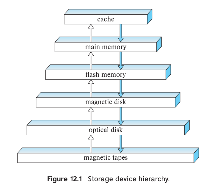
Media

• Cache
• Main memory
• Flash memory
• Magnetic-disk storage
• Optical storage
• Tape storage

Storage Interfaces

• Serial ATA (SATA)

  • SATA-3: nominally supports 6 GB/s, allowing data transfer speeds of up to 600 MB/s.

• Serial Attached SCSI (SAS): typically used only in servers.

  • SAS-3: nominally supports data transfer rates of 12 GB/s.

• Non Volatile Memory Express (NVMe): logical interface standard developed to better support SSDs and is typically used with the PCIe interface.

• Storage Area Network (SAN): large numbers of disks are connected by a high-speed network to a number of server computers. e.g. RAID.

  • iSCSI: An interconnection technology allows SCSI commands to be sent over an IP network.
  • Fiber Channel FC: supports transfer rates of 1.6 to 12 GB/s, depending on the version.
  • InfiniBand: provides very low latency high-bandwidth network communication.

• Network attached storage (NAS): provides a file system interface using networked file system protocols such as NFS or CIFS. e.g. cloud storage.

Magnetic Disks

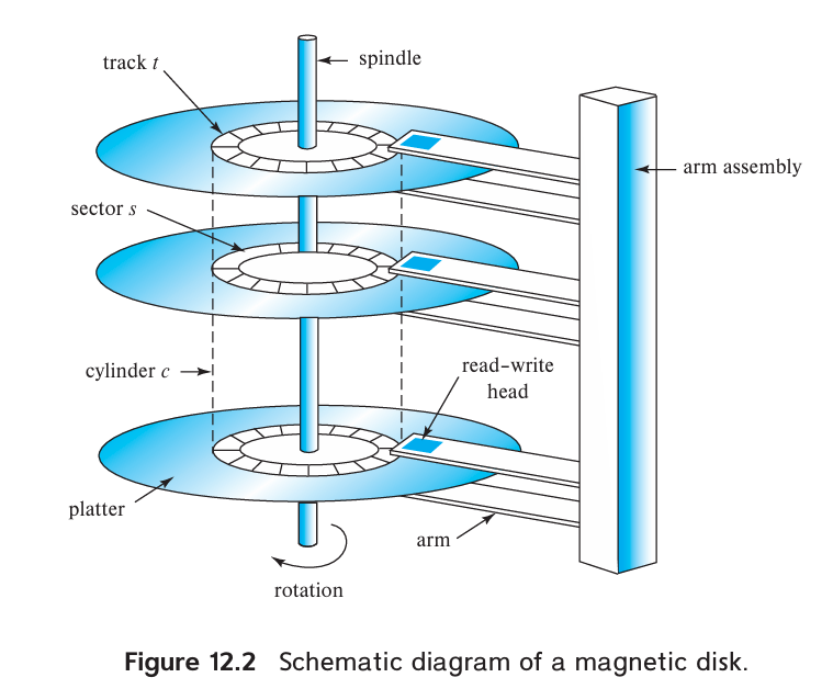
Performance Measurement

• Access time: The time from when a read or write request is issued to when data transfer begins, mainly include seek time and rotational latency time.
  • Seek time: The time for repositioning the arm. Typical seek times range from 2 to 20 milliseconds depending on how far the track is from the initial arm position. Average seek times currently range between 4 and 10 milliseconds, depending on the disk model.
  • Rotational latency time: The time spent waiting for the sector to be accessed to appear under the head. Typically range from 2 to 5.5 milliseconds.
• Data-transfer rate: The rate at which data can be retrieved from or stored to the disk. Current disk systems support maximum transfer rates of 50 to 200 MB/s.
• IOPS: With a 4KB block size, current generation disks support between 50 and 200IOPS, depending on the model.
• Mean time to failure (MTTF): According to vendors’ claims, the mean time to failure of disks today ranges from 500,000 to 1,200,000 hours—about 57 to 136 years.

Flash Memory

• Erase block: Once written, a page of flash memory cannot be directly overwritten. It has to be erased and rewritten subsequently. The erase operation must be performed on a group of pages, called an erase block.
• Translation table: Flash memory systems limit the impact of both the slow erase speed and the update limits by mapping logical page numbers to physical page numbers. The page mapping is replicated in an in-memory translation table for quick access.
• Wear leveling: Distributing erase operations across physical blocks, usually performed transparently by flash-memory controllers.
• Flash translation layer: All the above actions are carried out by a layer of software called the flash translation layer; above this layer, flash storage looks identical to magnetic disk storage, pro viding the same page/sector-oriented interface.

Performance Measurement

• IOPS: Typical values in 2018 are about 10,000 random reads per second with4KB blocks, although some models support higher rates.
• QD-n: SSDs can support multiple random requests in parallel, with 32 parallel requests being commonly supported (QD-32); a flash disk with SATA interface supports nearly 100,000 random 4KB block reads in a second with 32 requests sent in parallel, while SSDs connected using NVMe PCIe can support over 350,000 random 4KB block reads per second.
• Data transfer rate: Typical rates for both sequential reads and sequential writes are 400 to 500 megabytes per second for SSDs with a SATA 3 interface, and 2 to 3 GB/s for SSDs using NVMe over the PCIe3.0x4 interface.
• Random block writes per second: Typical values in 2018 are about 40,000 random 4KB writes per second for QD-1 (without parallelism), and around 100,000 IOPS for QD-32.

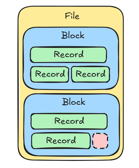
#13 Data Storage Structures

File Organization

File -> Block (fixed size, 4 to 8KB) -> Record (fixed or variable size)

Fixed-Length Records

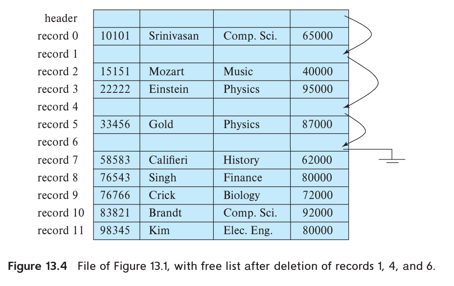
File header stores there is the address of the first record whose contents are deleted. The first record to store the address of the second available record, and so on. The deleted records thus form a linked list, which is often referred to as a free list.

Insertion and deletion can be easily done according to free list.

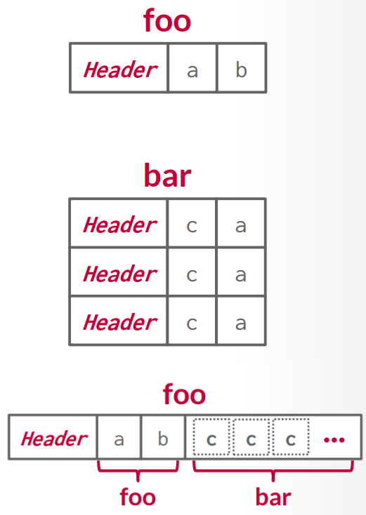
Variable-Length Records

For the presence of variable length fields, we use variable-length records.

A variable-length record looks like:

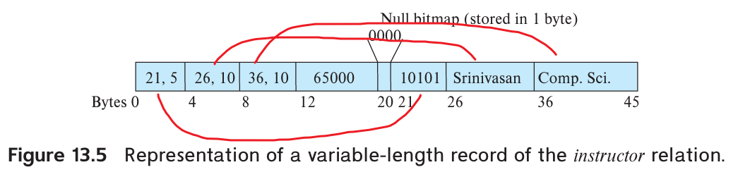
Variable-length attributes are represented in the initial part of the record by a pair (offset, length). The values for the variable-length attributes are stored consecutively, after the initial fixed-length part of the record.

Null bitmap indicates which attributes of the record have a null value.

The slotted-page structure is commonly used for organizing records within a block:

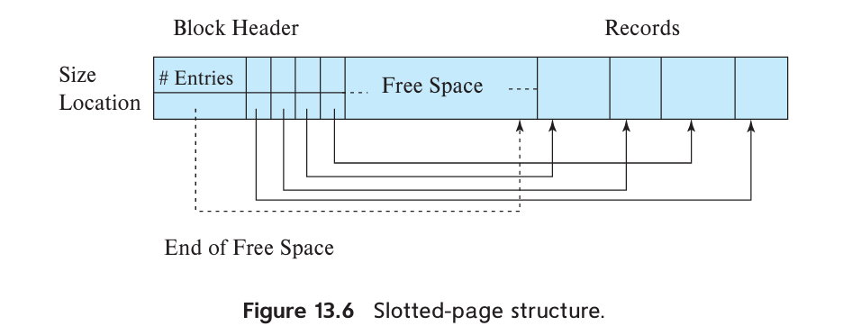
There is a header at the beginning of each block, containing the following information:

• The number of record entries in the header
• The end of free space in the block
• An array whose entries contain the location and size of each record

When a record is deleted, the space it occupied is freed up and its entry is marked as deleted (e.g. size set to -1). Additionally, the records in the block before the deleted record are shifted to fill the empty space created by the deletion. The cost of moving records is not too high because the block size is limited, typically around 4 to 8KB.

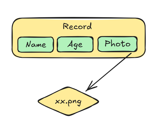
Storing Large Objects

Large objects may be stored either as files in a file system area managed by the database, or as file structures (e.g. B+ tree) stored in and managed by the database. A (logical) pointer to the object is then stored in the record containing the large object.

Organization of Records in Files

Heap file organization

In a heap file organization, a record can be stored anywhere in the file that corresponds to a relation. Once placed in a specific location, the record is typically not moved.

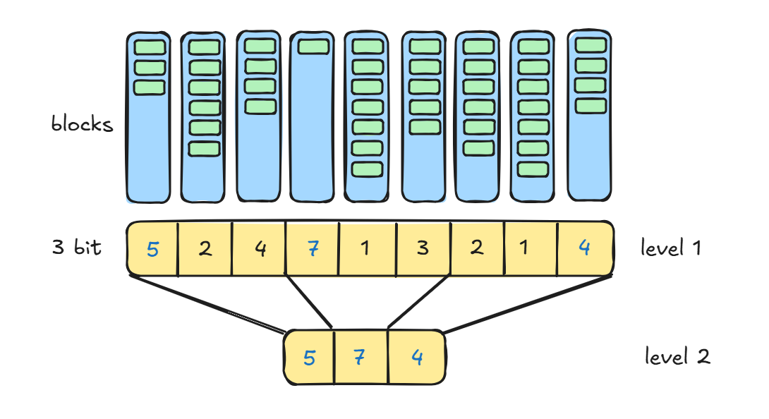
To implementing efficient insertion, most database use a space-efficient data structure called a free-space map to track which blocks have free space to store records.

The free-space map is commonly represented by an array containing 1 entry for each block in the relation. Each entry represents a fraction f such that at least a fraction f of the space in the block is free. Assume that 3 bits are used to store the occupancy fraction; the value at position i should be divide by 8 to get the free-space fraction for block i.

To find a block to store a new record of a given size, the database can scan the free-space map to find a block that has enough free space to store that record. If there is no such block, a new block is allocated for the relation.

For large files, it can still be slow to scan free-space map. To further speed up the task of locating a block with sufficient free space, we can create a second-level free-space map, which has, say 1 entry for every 100 entries for the main free-space map. That 1 entry stores the maximum value amongst the 100 entries in the main free-space map that it corresponds to. (Seems like a skip list :D) We can create more levels beyond the second level, using the same idea.

Sequential file organization

A sequential file is designed for efficient processing of records in sorted order based on some search key. A search key is any attribute or set of attributes. To permit fast retrieval of records in search-key order, we chain together records by pointers. The pointer in each record points to the next record in search-key order. Furthermore, to minimize the number of block accesses in sequential file processing, we store records physically in search-key order, or as close to search-key order as possible.

Maintaining physical sequential order is difficult when inserting or deleting records, as moving many records due to a single change is costly.

For insertion, we apply two rules:

1. Locate the record in the file that precedes the record to be inserted in search key order.
2. If there is available space in the same block, insert the new record there. Otherwise, insert the new record in an overflow block. In either case, adjust the pointers so as to chain together the records in search-key order.

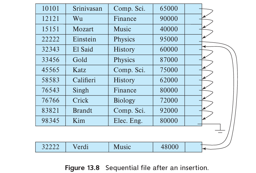
Reorganizing is still necessary if the overflow blocks become too large. To keep the correspondence between search-key order and physical order. (B+-tree file organization provides efficient ordered access even if there are many inserts, deletes, without requiring expensive reorganizations).

Multitable clustering file organization

Multitable clustering file organization stores related records of two or more relations in each block. The cluster key is the attribute that defines which records are stored together.

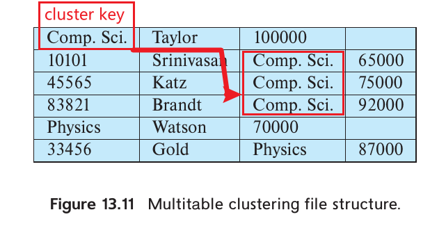
A multitable clustering file organization can speed up certain join queries but may slow down other types of queries.

The Oracle database system supports multitable clustering. Clusters are created using a create cluster command with a specified cluster key. The create table command extension can specify that a relation is stored in a specific cluster, using a particular attribute as the cluster key, allowing multiple relations to be allocated to one cluster.

B+-tree file organization

B+-tree file organization allows efficient ordered access even with numerous insertions, deletions, or updates while also enabling very efficient access to specific records based on the search key.

Detailed information will be discussed in #14.

Hasing file organization

A hash function is calculated based on a specific attribute of each record, determining the block in which the record should be stored in the file.

Detailed information will be discussed in #14.

Partitioning

Many databases allow records in a relation to be partitioned into smaller relations stored separately. Table partitioning is usually based on an attribute value, such as partitioning transaction records by year into separate relations for each year (e.g., transaction 2018, transaction 2019).

Table partitioning can avoid querying records with mismatched attributes. For example, a query select * from transaction where year=2019 would only access the relation transaction_2019.

Partitioning can help reduce costs for operations like finding free space for a record, as the size of relations increases. It can also be used to store different parts of a relation on separate storage devices. For example, in 2019, older transactions could be stored on magnetic disk while newer ones are stored on SSD for faster access.

#14 Indexing

Write-Optimized Index Structures

LSM Trees

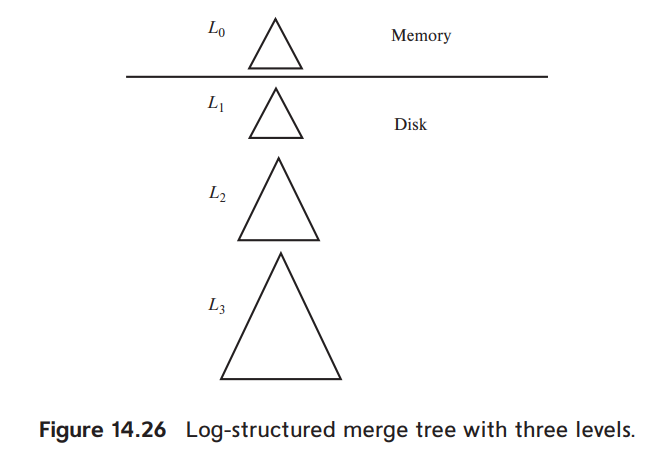
An LSM tree consists of several B+-trees (While it may not be a B+-tree like LevelDB, it is simply an ordered data structure), starting with an in memory tree, called L0 and on-disk L1, L2, ..., Lk, where k is called the level.

Lookup operation is performed by merging all lookup operations on each of the tree.

When a certain level is filled, it will be copied and form a new tree to be placed in the next level.

Each level except L0 could have multiple B+-trees, which is called stepped-merge index. The stepped-merge index decreases the insert cost significantly compared to having only one tree per level, but it can result in an increase in query cost.

Deletion results in insertion of a new delete entry that indicated which index entry is to be deleted. If a deletion entry is found, the to-be-deleted entry is filtered out and not returned as part of the lookup result.

When trees are merged, if one of the trees contains an entry, and the other had a matching deletion entry, the entries get matched up during the merge (both would have the same key), and are both discarded. Updates follow a similar procedure, only the newest entry will be returned as lookup result and kept during the merge.

LSM trees were originally created to decrease the write and seek overheads of magnetic disks. Flash-based SSDs have a lower overhead for random I/O operations because they do not need seeking, so the advantage of avoiding random I/O that LSM tree variations offer is not as crucial with SSDs.

However, the flash memory does not allow in-place update, writing even a single byte to a disk page requires the whole page to be rewritten to a new physical location (The original location of the page needs to be erased firstly). Using LSM tree variants could reduce the number of writes and decrease the wearing rate.

Many BigData storage systems, including Apache Cassandra, Apache AsterixDB, and MongoDB, now support LSM trees. MySQL (with the MyRocks storage engine), SQLite4, and LevelDB also offer support for LSM trees.

#24 Advanced Indexing Techniques

Log-Structured Merge Tree and Variants

Insertion into LSM Trees

Lectures

Lectures notes and thoughts

• CMU 15445 Intro to Database Systems

CMU 15445 Intro to Database Systems

#01 Relation Model & Algebra

1. Concepts

• A database is an organized collection of inter-related data that models some aspect of the real-world.
• A data model is a collection of concepts for describing the data in database.
  • Relation (most common)
  • NoSQL (kv, doc, graph)
  • Array / Matrix / Vector (for ML)
• A schema is a description of a particular collection of data, using a given data model.
  • This defines the structure of data for a data model
  • Otherwise, you have random bits with no meaning

2. Relation Algebra

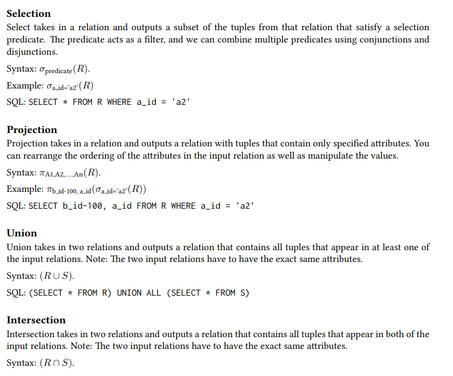
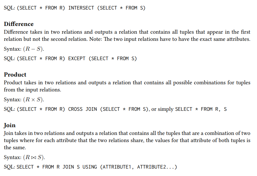
#02 Modern SQL

1. Relation Languages

• Data Manipulation Language (DML)
  • SELECT, UPDATE, DELETE, ...
• Data Define Language (DDL)
  • CREATE ...
• Data Control Language (DCL)
  • GRANT ...

2. Aggregates

• AVG(COL): The average of the values in COL
• MIN(COL): The minimum value in COL
• MAX(COL): The maximum value in COL
• SUM(COL): The sum of the values in COL
• COUNT(COL): The number of tuples in the relation

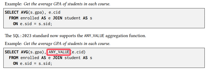
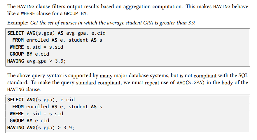
3. String Operations

The SQL standard says that strings are case sensitive and single-quotes only. There are functions to manipulate strings that can be used in any part of a query.

Pattern Matching: The LIKE keyword is used for string matching in predicates.

• “%” matches any substrings (including empty).
• “_” matches any one character.

Examples of standard string functions include SUBSTRING(S, B, E) and UPPER(S).

Concatenation: Two vertical bars (“||”) will concatenate two or more strings together into a single string.

4. Date and Time

Databases generally want to keep track of dates and time, so SQL supports operations to manipulate DATE and TIME attributes. These can be used as either outputs or predicates.

Specific syntax for date and time operations can vary wildly across systems.

5. Output Control

• ORDER BY <column> [ASC|DESC]
• FETCH [FIRST|{NEXT}] <count> ROWS ONLY {OFFSET <count>} {WITH TIES} (ANSI SQL)
  • LIMIT <count> OFFSET <count> (MySQL/SQLite)

> SELECT * FROM employee;

|name|salary|
-------------
| A  | 1000 |
| B  | 1300 |
| C  | 1100 |
| D  | 1100 |
| E  | 1400 |

> SELECT salary FROM employee FETCH FIRST 3 ROWS WITH TIES;

|salary|
--------
| 1000 |
| 1300 |
| 1100 |
| 1100 | <- TIES

6. Window Functions

A window function performs “sliding” calculation across a set of tuples that are related. Window functions are similar to aggregations, but tuples are not collapsed into a singular output tuple.

Aggregations:

|name|salary|age|
-----------------
| A  | 1000 |23 |
| B  | 1300 |22 |
| C  | 1100 |23 |
| D  | 1100 |45 |
| E  | 1400 |22 |

--- Aggregate by age ---

|name |salary     |age|
-----------------------
| A,C | 1000,1100 |23 |
| B,E | 1300,1400 |22 |
| D   | 1100      |45 |

--- Mean on salary ---

|salary|age|
------------
| 1050 |23 |
| 1350 |22 |
| 1100 |45 |

Window:

|name|salary|age|
-----------------
| A  | 1000 |23 |
| B  | 1300 |22 |
| C  | 1100 |23 |
| D  | 1100 |45 |
| E  | 1400 |22 |

--- Window over age ---

|name|salary|age|
-----------------
| A  | 1000 |23 |
| C  | 1100 |23 |
-----------------
| B  | 1300 |22 |
| E  | 1400 |22 |
-----------------
| D  | 1100 |45 |

--- ROW_NUMBER()/RANK(salary) ---

|name|salary|age|row_number
---------------------------
| A  | 1000 |23 |1
| C  | 1100 |23 |2
---------------------------
| B  | 1300 |22 |1
| E  | 1400 |22 |2
---------------------------
| D  | 1100 |45 |1

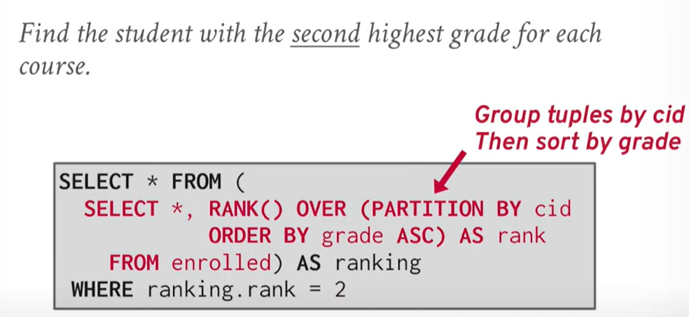
7. Nested Queries

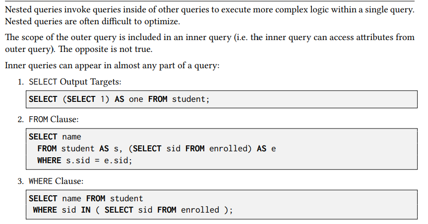
Nested Query Results Expressions:

• ALL: Must satisfy expression for all rows in sub-query.
• ANY: Must satisfy expression for at least one row in sub-query.
• IN: Equivalent to =ANY().
• EXISTS: At least one row is returned

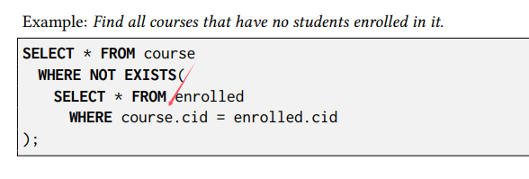
8. Lateral Joins

The LATERAL operator allows a nested query to reference attributes in other nested queries that precede it. You can think of lateral joins like a for loop that allows you to invoke another query for each tuple in a table.

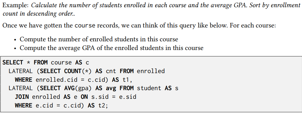
SELECT * FROM course AS c,

|cid   |name    
-------------       
|15-445|Database System
|15-721|Advanced Database System
|15-826|Data Mining

LATERAL (SELECT COUNT(*) AS cnt FROM enrolled
          WHERE enrolled.cid = c.cid) AS t1,

-- For each cid in c, execute
-- `SELECT COUNT(*) AS cnt FROM enrolled WHERE enrolled.cid = c.cid`

|cid   |name                    |cnt
------------------------------------
|15-445|Database System         |2
|15-721|Advanced Database System|3
|15-826|Data Mining             |2

-- 

LATERAL (SELECT AVG(gpa) AS avg FROM student AS s
           JOIN enrolled AS e ON s.sid = e.sid
          WHERE e.cid = c.cid) AS t2;

-- For each cid in c, execute
-- `SELECT AVG(gpa) AS avg FROM student AS s JOIN enrolled AS e ON s.sid = e.sid WHERE e.cid = c.cid`

|cid   |name                    |cnt|avg
----------------------------------------
|15-445|Database System         |2  |3.2
|15-721|Advanced Database System|3  |3.4
|15-826|Data Mining             |2  |3.6

9. Common Table Expressions

Common Table Expressions (CTEs) are an alternative to windows or nested queries when writing more complex queries. They provide a way to write auxiliary statements for use in a larger query. A CTE can be thought of as a temporary table that is scoped to a single query.

WITH cteName AS (
    SELECT 1
)
SELECT * FROM cteName;

|*|
---
|1|

Bind output columns to names before the AS:

WITH cteName (col1, col2) AS (
    SELECT 1, 2
)
SELECT col1 + col2 FROM cteName;

Multiple CTE declarations in single query:

WITH cte1 (col1) AS (SELECT 1), cte2 (col2) AS (SELECT 2)
SELECT * FROM cte1, cte2;

Adding the RECURSIVE keyword after WITH allows a CTE to reference itself. This enables the implementation of recursion in SQL queries. With recursive CTEs, SQL is provably Turing-complete, implying that it is as computationally expressive as more general purpose programming languages (ignoring the fact that it is a bit more cumbersome).

Print the sequence of numbers from 1 to 10:

WITH RECURSIVE cteSource (counter) AS (
    ( SELECT 1 )
    UNION
    ( SELECT counter + 1 FROM cteSource
        WHERE counter < 10 )
)
SELECT * FROM cteSource;

select c.name as COACH_NAME, count(*) as MEDAL_NUMBER 
  from coaches as c
    join (
      select m.discipline, t.country_code from medals as m join 
        (
          select code, country_code from teams 
          union all
          select code, country_code from athletes
        ) as t on m.winner_code = t.code
    ) as o on c.country_code = o.country_code
    and c.discipline = o.discipline
    group by c.name 
    order by MEDAL_NUMBER desc, COACH_NAME;

with medals_cnt as ( -- athlete_code, cnt
  select athlete_code, sum(cnt) as cnt from
    (select athletes.code as athlete_code, count(*) as cnt
      from athletes, medals 
        where athletes.code = medals.winner_code
      group by athletes.code
    union all -- row duplicated is allowed
    select athletes_code as athlete_code, count(*) as cnt
      from teams, medals
        where teams.code = medals.winner_code
      group by athletes_code)
  group by athlete_code
)
select name as ATHLETE_NAME, 
  (case when cnt is not null then cnt else 0 end) as MEDAL_NUMBER 
  from athletes left join medals_cnt -- use left join to keep all records in athletes
    on athletes.code = medals_cnt.athlete_code 
  where athletes.disciplines like '%Judo%' 
  order by MEDAL_NUMBER desc, ATHLETE_NAME;

with comp as (
  select participant_code, participant_type
      from results, venues
      where results.venue = venues.venue 
        and venues.disciplines like '%Athletics%'
), a as (
  select *
  from athletes
  where code in 
      (select distinct participant_code
      from 
          (select participant_code 
          from comp 
          where participant_type = 'Person'
          union
          select athletes_code as participant_code 
          from teams, comp
          where comp.participant_type = 'Team' 
            and comp.participant_code = teams.code))
)
select 
    name as ATHLETE_NAME, 
    country_code as REPRESENTED_COUNTRY_CODE, 
    nationality_code as NATIONALITY_COUNTRY_CODE
from 
    (select t.*, countries.Latitude as nationality_latitude, countries.Longitude as nationality_longitude
    from 
        (select a.*, countries.Latitude as country_latitude, countries.Longitude as country_longitude 
        from a left join countries on a.country_code = countries.code) as t 
        left join countries on t.nationality_code = countries.code
    where nationality_latitude is not null 
          and nationality_longitude is not null 
          and country_latitude is not null 
          and country_longitude is not null)
order by 
    (country_latitude - nationality_latitude)^2 + (country_longitude - nationality_longitude)^2 desc, athlete_name;

with country_rank as (
select
    code,
    rank() over (order by "GDP ($ per capita)" desc) as gdp_rank,
    rank() over (order by "Population" desc) as population_rank
from
    countries
)
select 
  t1.date as DATE,
  t1.country_code as COUNTRY_CODE,
  t1.cnt as TOP5_APPEARANCES,
  country_rank.gdp_rank as GDP_RANK,
  country_rank.population_rank as POPULATION_RANK
from 
  (select *,
    row_number() over (partition by date order by date, cnt desc) as row_number 
    from (
      select date,
       country_code,
       count(*) as cnt
      from (
        select date, rank, country_code 
        from results, athletes 
        where results.participant_type = 'Person' 
          and results.participant_code = athletes.code
        union all
        select date, rank, country_code
        from results, teams 
        where results.participant_type = 'Team'
          and results.participant_code = teams.code)
    where rank <= 5 group by date, country_code)) as t1, country_rank
where t1.row_number = 1 and country_rank.code = t1.country_code
order by date;

with t as (
	select code, country_code from teams group by code, country_code
) -- team may duplicate
select * from (
  select
    t1.country_code as COUNTRY_CODE,
    t1.paris_gold - t2.gold_medal as INCREASED_GOLD_MEDAL_NUMBER,
  from (
    select
      country_code,
      count(*) as paris_gold
    from (
      select country_code
      from medals, athletes 
      where medals.winner_code = athletes.code and medal_code = 1
      union all
      select country_code
      from medals, t
      where medals.winner_code = t.code and medal_code = 1
    )
    group by country_code
  ) as t1, tokyo_medals as t2
  where t1.country_code = t2.country_code
  order by INCREASED_GOLD_MEDAL_NUMBER desc
  limit 5
) as i1,
lateral (
  select teams.code as TEAM_CODE
  from teams, athletes
  where teams.athletes_code = athletes.code and teams.country_code = i1.country_code
  group by teams.code
  having SUM(1- gender) = 0 -- mem: 0, women: 1 [all female = 'sum(1 - gender) = 0']
)
order by INCREASED_GOLD_MEDAL_NUMBER desc, COUNTRY_CODE, TEAM_CODE;

#03 Database Storage: Files & Pages

1. Storage Interface

Overview:

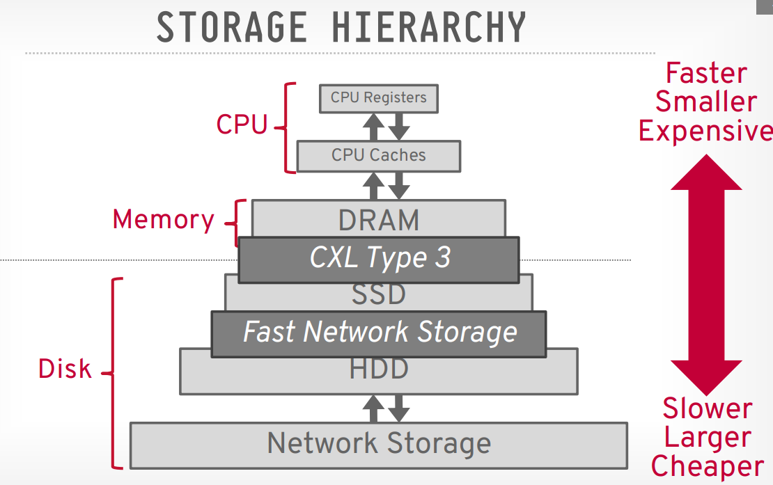
Access time comparation:

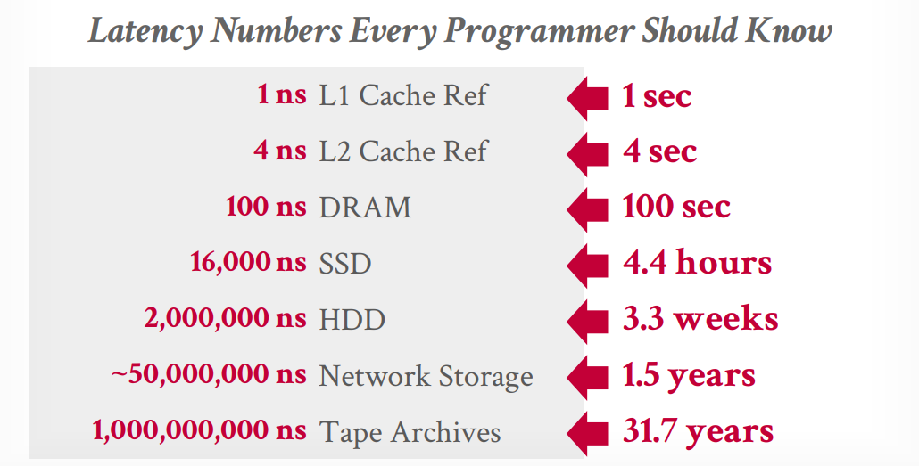
2. Use mmap or not?

• You never want to use mmap in your DBMS if you need to write.
• The DBMS (almost) always wants to control things itself and can do a better job at it since it knows more about the data being accessed and the queries being processed.

But it is possible to use by using:

• madvise: Tells the OS know when you are planning on reading certain pages.
• mlock: Tells the OS to not swap memory ranges out to disk.
• msync: Tells the OS to flush memory ranges out to disk.

Even though the system will have functionalities that seem like something the OS can provide, having the DBMS implement these procedures itself gives it better control and performance.

3. Files

In its most basic form, a DBMS stores a database as files on disk. Some may use a file hierarchy, others may use a single file (e.g., SQLite).

The DBMS’s storage manager is responsible for managing a database’s files. It represents the files as a collection of pages. It also keeps track of what data has been read and written to pages as well how much free space there is in these pages (e.g. free-space map).

4. Pages

• Fixed-size: Typically 4 to 16KB. Most DBMSs uses fixed-size pages to avoid the engineering overhead needed to support variable-sized pages. We really don't want to deal with variable-sized pages after dealing with variable-sized records.

  • Read-only workloads may have larger page sizes.

• Self-contained: Some systems will require that pages are self-contained, meaning that all the information needed to read each page is on the page itself. This is very useful in disaster recovery, as it can still recover some data from the remaining half when half of the disk is damaged.

• Page Directory: DBMS maintains special pages, called page directory, to track locations of data pages, the amount of free space on each page, a list of free/empty pages and the page type. These special pages have one entry for each database object.

Every page includes a header that records metadata about the page's contents:

• Page size.
• Checksum.
• DBMS version.
• Transaction visibility.
• ...

There are serval ways to lay out records in a page:

• Slotted Pages

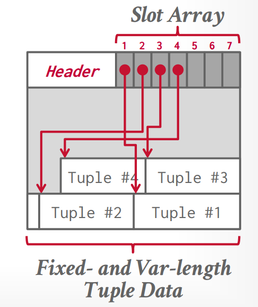
Header keeps track of the number of used slots, the offset of the starting location of the last used slot, and a slot array, which keeps track of the location of the start of each tuple.

To add a tuple, the slot array will grow from the beginning to the end, and the data of the tuples will grow from end to the beginning. The page is considered full when the slot array and the tuple data meet.

To delete a tuple, the entry in the slot array will be wiped out. We can shift the remaining tuples to maintain they are consecutive at the end of page.

• Log Structured

// Covered in the next lecture.

5. Tuples

Each tuple may have a tuple header to contains metadata about the tuple; it can be constructed of:

• Transaction visibility.
• Bitmap for NULL values.
• ...

Unique Identifier is required to identify a tuple and the most common format is page_id + (offset or slot)

• Denormalized Tuple Data: If two tables are related, the DBMS can “pre-join” them, so the tables end up on the same page. This makes reads faster since the DBMS only has to load in one page rather than two separate pages. However, it makes updates more expensive since the DBMS needs more space for each tuple.

#04 Database Storage: Log-Structured Merge Trees & Tuples